A Complete Guide on How to Remove Duplicates in Excel

Microsoft Excel is one of the best applications that Data Analysts use daily. Huge amounts of data are copied or imported on a regular basis from various excel files or from the internet, and it is now obvious that there will be a duplicate of the data as well. Because data is so important these days, it’s critical to understand how to remove only the duplicate entries while keeping the originals.
In this tutorial, we will show you 3 different methods for removing duplicate values in Excel, which are as follows:
- Use Remove Duplicates option
- Use Advanced Filter
- Use COUNTIF function
As shown in the screenshot below, we are going to walk you through all 3 of the different approaches on the sales data.
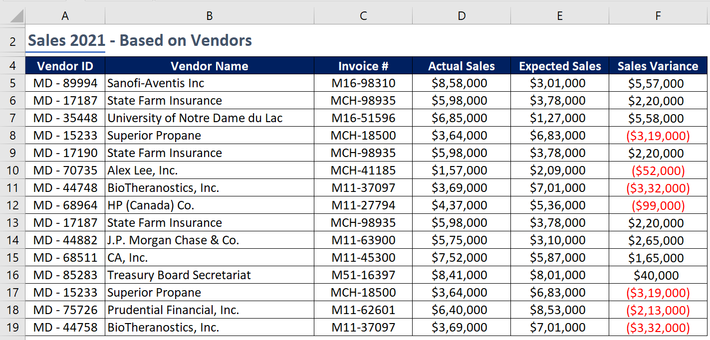
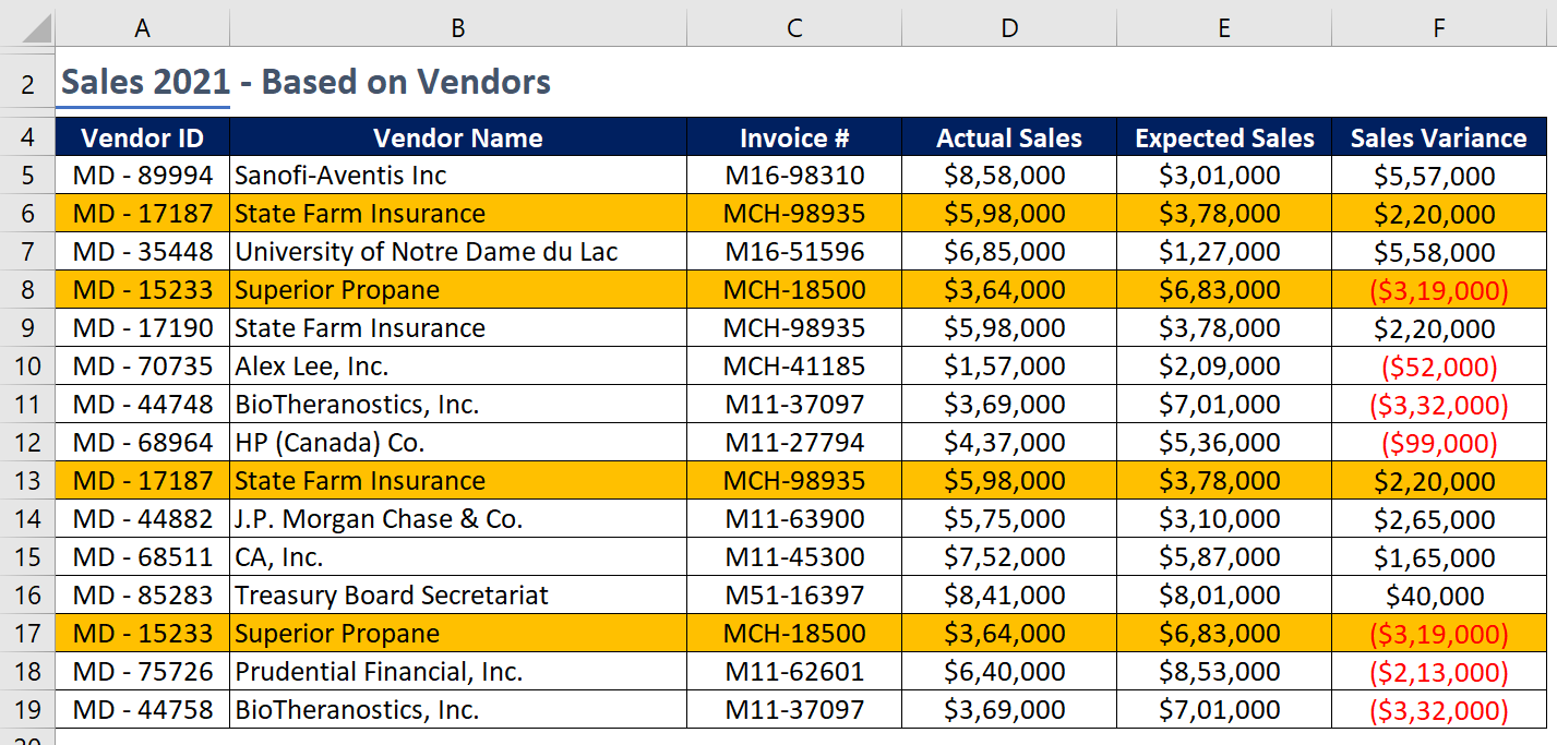
As you can see in the screenshot below, there are a total of 15 vendor entries, 4 of which are duplicates. Because the vendor IDs “MD – 17187” and “MD – 15233” appear twice, these 4 entries are highlighted.
Now, the task is to ensure that each entry appears only once, and if any vendor ID appears twice, the duplicate entry (row) must be deleted.
Here are the solutions to the problem presented above:
Option 1 – Use Remove Duplicates option
Excel includes a feature that allows you to remove duplicate entries. Follow the steps below:
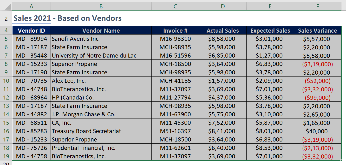
Step 1: Choose the only area you want to remove. We want to remove the entire duplicate row in this problem, so we will select the entire area from cell A4 to F19, including the heading, as shown in the screenshot below.
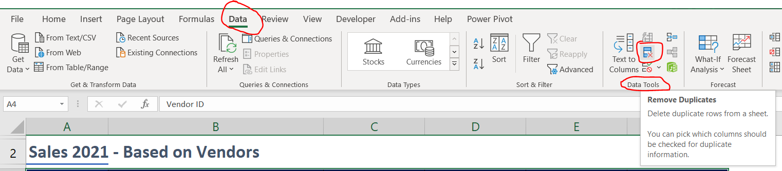
Step 2: Select the Remove Duplicates option by selecting one of the options listed below.
- Shortcut key: Alt + A + M
- Navigation: Data Tab > Data Tools Section > Remove Duplicates
Step 3: A Remove Duplicates dialogue box appears, as depicted in the image below.
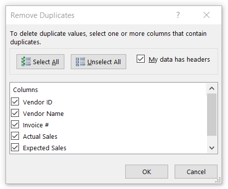
The above dialogue box will display a list of all the headings found in the data. Only those columns will be selected based on which we want to remove duplicate entries. However, in this case, we only want to remove duplicate rows based on the Vendor ID. So, we’ll click the Unselect All button and then check the Vendor ID checkbox only. Finally, the screenshot will look like this:
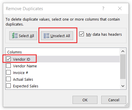
Then click on OK button.
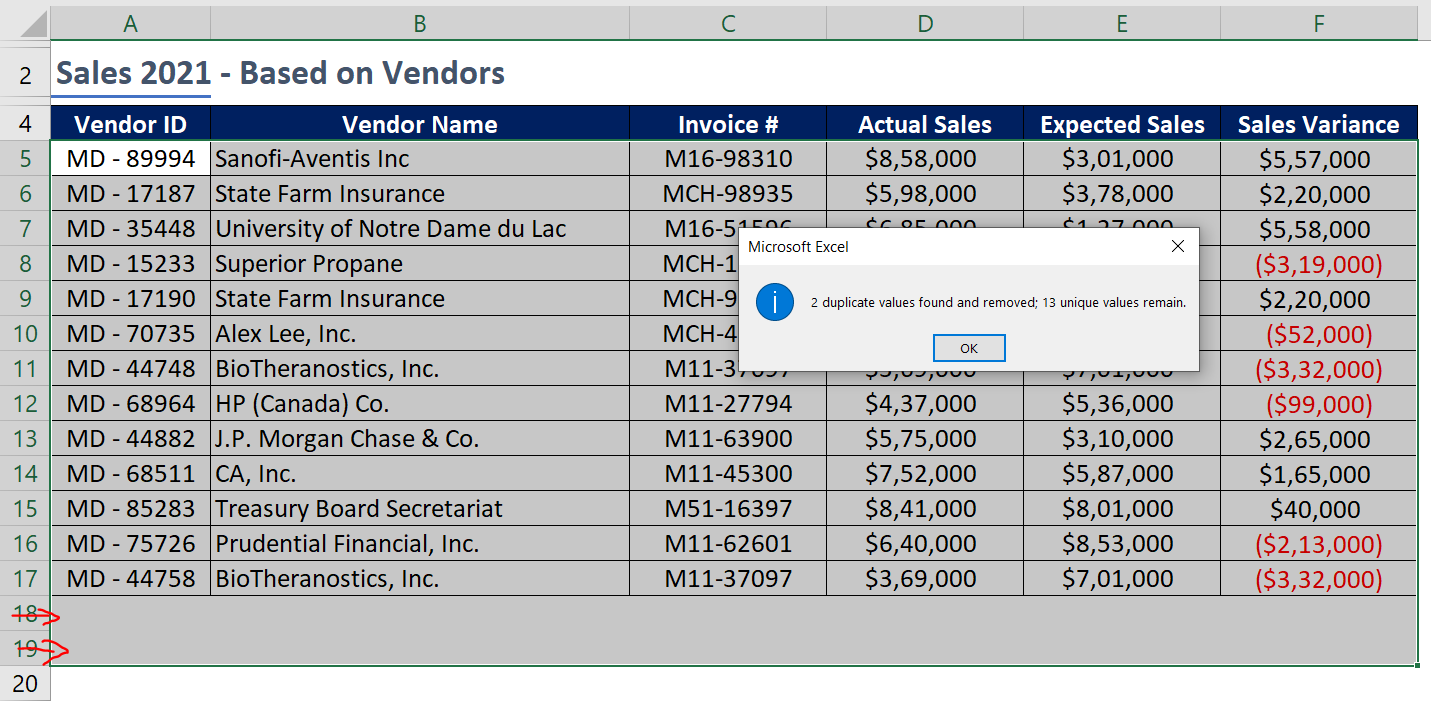
Step 4: When we click the OK button, we will see a message box stating that two duplicate values were discovered and removed. As we can see in the data, there are no entries in the 18th and 19th rows.
Option 2 – Use Advanced Filter
It’s possible that most Excel users have never heard of the Advanced Filter option, but it exists. Using this option, we can export data from one location to another based on unique entry conditions without affecting the original data which we are going to perform in this method.
Follow the below steps:
Step 1: Select the entire area from cell A4 to F19, including the heading, as shown in the screenshot below.
Step 2: Follow any of the following options to access the Advanced Filter:
- Shortcut key: Alt + A + Q
- Navigation: Data Tab > Sort & Filter Section > Advanced
Step 3: The Advanced Filter dialogue box appears, as shown in the screenshot below:
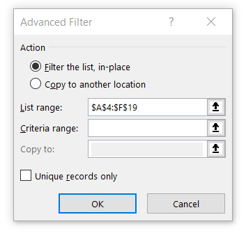
The above dialogue box displays various options, which I will explain one by one:
- Filter the list, in place: Select this option if you want to perform the action in the same location where the data is available.
- Copy to another location: Select this option if you want to perform the action and have the results delivered to a different location.
- List range: Select the range of complete data on which the action will be performed.
- Criteria range: If we have a specific criterion, only then will we select this option. This option will not be used for our problem.
- Copy to: This option is only enabled if the Copy to another location option is selected. In this option, you must choose a cell where you want the output.
- Unique records only: If the user wants only unique entries, or if he wants to remove duplicate entries, he must select this option; otherwise, identical data will be returned.
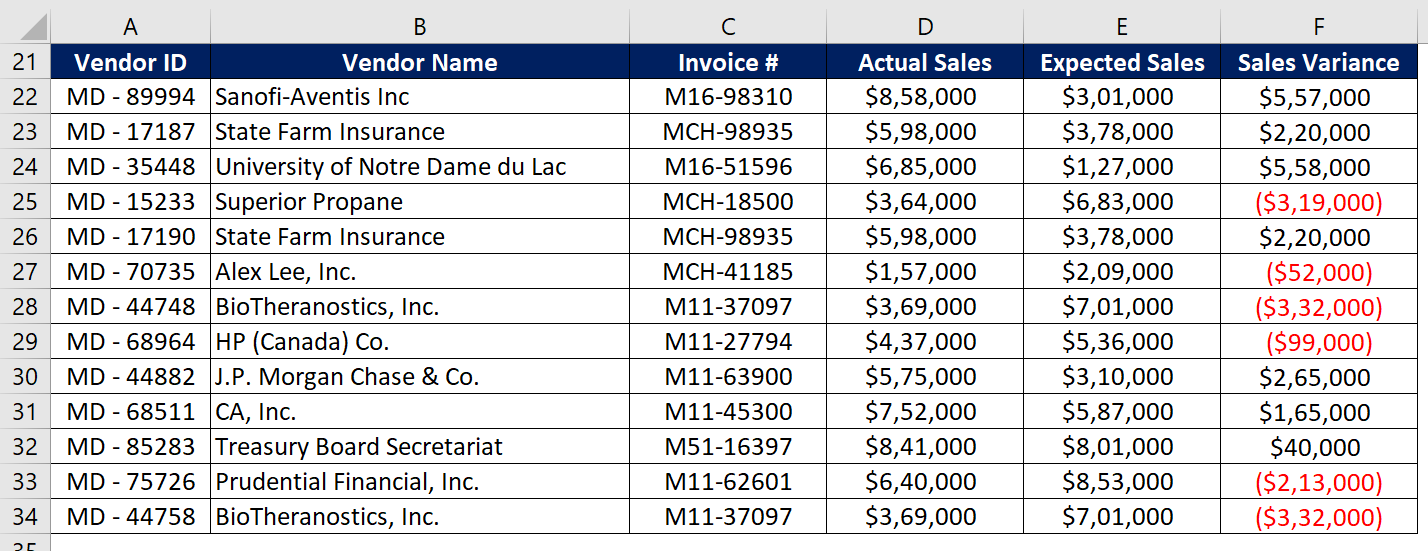
Step 4: Select the options shown in the screenshot below, then click the OK button.
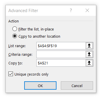
We have selected $A$21 cell in the Copy to option because we want the results from cell A21.
You will receive the results displayed in the image below.
Option 3 – Use COUNTIF Function
Excel’s COUNTIF function can be used to count the number of cells in a range that meet a given condition.
Follow the below steps:
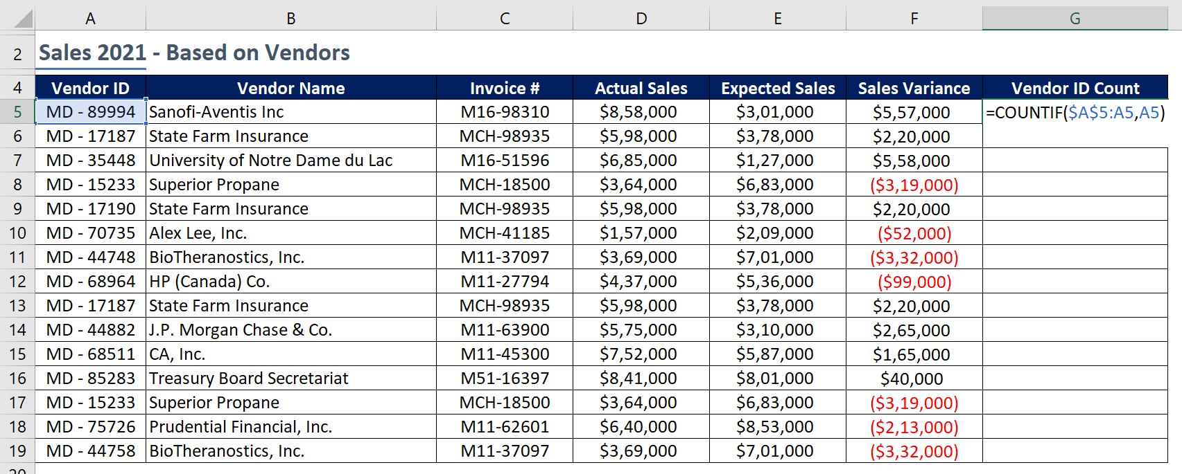
Step 1: Insert a new column titled “Vendor ID Count.”
Step 2: Write a COUNTIF formula as depicted in the image below to count the unique values based on the vendor ID column.
The key point is that you must freeze the value of the first A5 cell by using the dollar sign ($) or pressing the F4 key.
Step 3: Copy the formula from cell G5 and paste it into each of the empty cells G6 through G19. As depicted in the image below, there are two rows with a count of two and the remaining rows have a count of one. It indicates that these two rows contain duplicate entries.
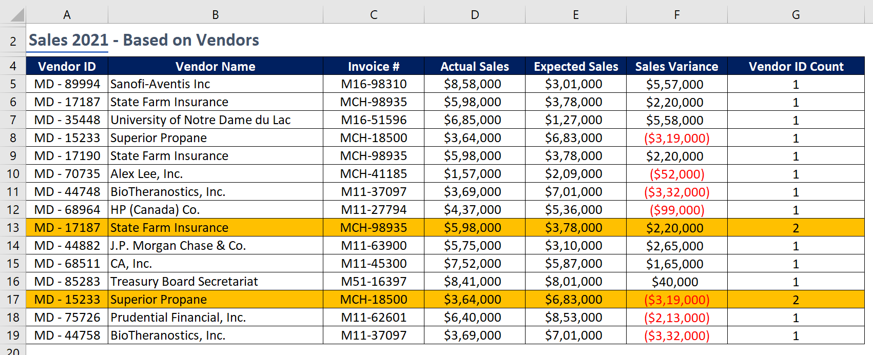
Step 4: We have currently highlighted the duplicate entries. If the data is small, we can manually remove rows where the count is 2. If the data set is very large, we can apply a number filter in column G that reads “is greater than 1” and then remove the available entries.
Conclusion:
When you remove duplicate values manually, not only will it take a significant amount of time, but there is also a chance that the user will make some mistakes. We have learned in this article the various methods that we can use in Excel to remove duplicate values. These methods can be applied in just a few seconds, which will save us a great deal of time.
Enhancing your knowledge of advanced features and functions of Microsoft Excel is something that Mdata Finnovatics can assist you with. You can check our latest blogs and YouTube videos for the same.
12 Responses
You’re so awesome! I don’t believe I have read a single thing like that before. So great to find someone with some original thoughts on this topic. Really.. thank you for starting this up. This website is something that is needed on the internet, someone with a little originality!
We appreciate your comment, Denzel. I’d like to know more about the kind of content you would like us to include on this site in order to attract more readers.
There is definately a lot to find out about this subject. I like all the points you made
Thank you for your kind appreciation! Please help us by sharing the website link with as many learners as possible. By doing so, they can empower their careers through the application of knowledge. We also welcome your suggestions for the next blog topic. Your input is valuable to us as we strive to provide relevant and engaging content.
Thanks!
A masterpiece! The way the author articulates thoughts is simply brilliant. Leaving with newfound knowledge and respect.
This is an excellent and informative post. The subject matter is captivating and extremely useful. Thank you for your efforts, admin. @Piroderler
Thank you for the content you share. Great topic and helpful. Thank you admin. Sevgilerle PİRO
This is really cool and helpful, Mekanbahis I don’t know if you believe it or not, but I follow here regularly.
This looks great, I will stay tuned for posts like this. Thank you.
Nice post! It was insightful and well-written, offering useful advice. Enjoyed reading it!
Great blog post! It provided valuable insights and practical tips. I found it very helpful and engaging.